Million Song Dataset Analysis

Team Members: Leonardo Tang, Sahir Shahryar

Introduction

Machine learning models have revolutionized the way we discover and listen to music. Much of the value that modern music streaming services provide to their users lies in their ability to recommend new music that users will enjoy listening to. However, we believe there may be more possible applications for machine learning when it comes to music. For our project, we'd like to explore two such applications: predicting hit songs, and classifying songs into genres.

Problem Definition

Supervised Learning: Hit Prediction

There has already been some research into using supervised learning techniques to classify songs’ emotion and artistic style [1, 2].

The MSD contains data about a song’s “hotness,” which is a measure of its short-term popularity at the time the song was added into the dataset [3, 4]. We set out trying to train a model that can predict, given every attribute except the hotness of a song, whether that song is a hit. In order to do this, we deliberately excluded a random sampling of songs from the dataset, trained the model on the remainder, and then tested how accurately the model predicted the hotness of the excluded songs. If such a model shows promise, it could theoretically be used to predict tomorrow’s hits.

Unsupervised Learning: Genre Classification

The complementary datasets to MSD contain genre labels, user data, etc. We would like to train a model that can assign songs to a specific genre. To do so, we will employ k-means clustering, GMM, DBSCAN, and spectral clustering. K-means is fast, but doesn’t allow for anything other than spherical clusters, so we will also attempt DBSCAN and spectral clustering to account for differently shaped clusters in the feature space [5]. GMM provides a soft clustering approach that will help smooth out data points that mix genres. In the event where clustering doesn’t seem to align to genres, a more general interpretation of the clusters would be music recommendations from a holistic view, determined by all the features of the song rather than just genre. This model should hopefully return the genre of the song, and if not, the clusters in the model can be used for song recommendations.

Data Collection

The researchers behind the Million Song Dataset provided a 1% sample of the dataset (i.e., 10,000 songs) that was available for download directly from their website. We used this dataset for the midterm report. However, downloading the rest of the dataset would prove very cumbersome. The full dataset, which is roughly 280 GB in size, must be downloaded using an Amazon EC2 instance. We created an AWS account for this purpose and used several copies of the `rsync` Unix utility running in parallel to clone parts of the dataset. After downloading roughly 10% of the dataset (around 116,900 songs), we decided to stop, as downloading only that much of the data incurred a $12 bill from Amazon.

The data itself was presented using HDF5 (hierarchical data format) files, which required us to install special libraries to even open the dataset. We used wrapper code provided by the authors of the MSD to iterate through the HDF5 files and convert some of the features inside into a CSV format. We chose to include the following features for the *unsupervised* portion of the project:

Some of the features we chose to discard for this portion of the project include the following:

For the unsupervised portion of our project (genre classification), we wanted to include the timbre of the song as a feature. We were interested in seeing whether there is some correlation between the sound profile of a song and the genre it belongs to. However, as mentioned above, the timbre is provided as a large matrix which cannot be easily used as a feature on its own. While trying to understand the values inside this matrix, we fell into a rabbit hole about MFCCs — mel-frequency cepstral coefficients — which are the way in which the MSD encodes timbre information. In a nutshell, rather than using plain frequency data (measured in Hz) and encoding that information into the dataset, the authors of the MSD converted the frequency data into mels, which essentially applies a log function to the frequency data. This is done because human perception of pitch is itself logarithmic, meaning that the perceived difference between a 440 Hz tone and a 640 Hz tone is larger than the perceived difference between a 2440 Hz tone and a 2640 Hz tone, even though they are both 200 Hz apart. Interestingly, we learned that conversion to mels is used for voice-recognition applications as well [7].

To fit the timbre data into a fixed number of features, we decided to use a strategy similar to a Markov chain. The intent behind doing this was trying to come up with a metric for how the song “flows,” in a sense, rather than just averaging the frequencies across the entire song.

The unfiltered timbre data was provided as an N-by-12 matrix, where N depends on the length of the song. For each row of the matrix (i.e. the timbre information at a given time in the song), we chose the range of frequencies that were the loudest. We then counted the number of transitions the song made between these loudest frequencies. This created a matrix where, at cell i,j, we counted how many times the song went from having frequency band i as its loudest frequency to having frequency band j as its loudest frequency immediately afterwards. After dividing each row by the number of sum of all values on that row, we end up with the matrix of a Markov chain which contains probabilities rather than raw counts. Unfortunately, with 12 frequency bands, there are still too many features (at 144), so we averaged together pairs of frequency bands to end up with six frequency ranges and 36 total features.

For the genre ground truth labels, we use the MSD Allmusic Top Genre Dataset, which had the top genre labels for 406,627 different tracks. The genres are as follows:

Methods

Supervised Learning:

Logistic Regression:

For logistic regression, the features that we chose were duration, key, loudness, mode, tempo, time signature, artist familiarity, and artist hotness. 80% of the songs were set aside as training data while the remaining 20% were used for testing purposes. For our labels, we based them on the song hotness column, splitting the songs into two categories, “hit” or “not hit” based on their song hotness values. Any song with a song hotness value above the sample mean was deemed a hit, while any song with a song hotness value below the sample mean was deemed not a hit.

Naive Bayes:

We also tried using naive Bayes to classify songs as either a hit or not a hit (using the same rule as for logistic regression). First, to reduce the number of features being used, we used k-best feature selection, with the scoring metric being an analysis of variance. (We also tried using χ^2, but this was not suitable as loudness values are stored in decibels (dB), which can be negative.) Using these features, we used sklearn’s GaussianNB class to test the model, with 80% of the data being used for training and 20% for testing.

Neural Networks:

After learning more about neural networks in class, we also tried using a simple neural network for this problem. We assembled a dense neural network with TensorFlow’s Keras library, trying a variety of layer sizes and activation functions for each layer. (For example, we tried training a network with two hidden layers with 20 and 10 nodes respectively.)

Unsupervised Learning:

We employed 3 different clustering methods to attempt genre classification of the Million Song Dataset. While the clustering itself was done without any labels, the ground truth labels were taken from the MSD Allmusic Top Genre Dataset. The methods we used were K-Means, Gaussian Mixture Models, and DBScan. Each method was run on two datasets, one with the timbre features and one without. We reasoned that the timbre data might help with clustering the data, but we also wanted to keep a control group without the timbre data in case that might work better.

K-Means:

The first clustering model we used was K-Means. To get the optimal k value, we ran a K-Means models for 2 clusters up to 14 clusters and plotted the loss values so that we could use the elbow method determine the best k value. The loss was defined as the sum of squared errors. As additional insurance, we also modeled the silhouette values for each k value in case the graph outputted by the elbow method was not clear where the optimal k value should be. After finding the optimal k value, we determined the cluster distribution for each genre, i.e. for each genre that exists within the dataset, we counted up the number of data points that were sent to each cluster. Doing this would allow us to see if there were any genres that seemed to be overwhelmingly assigned to a specific cluster.

Gaussian Mixture Model (GMM):

We repeated the same process for GMM. The reason why we decided to include GMM was that K-Means is spherical and would therefore be inaccurate if the optimal clusters in the data were not spherical. GMM would allow us to model ellipsoidal clusters, giving us the option to put less weight on features that were less important.

DBScan:

DBScan would allow us to have irregularly shaped clusters that do not fit the spherical cluster model or the Gaussian cluster model. For DBScan, we had to tune the epsilon and minimum samples parameters. Concretely, we tested parameters from 0.5 to 2.0 in 0.05 increments.

Results and Discussion

Supervised Learning

Logistic Regression:

For logistic regression, the features that we chose were duration, key, loudness, mode, tempo, time signature, artist familiarity, and artist hotness. 80% of the songs were set aside as training data while the remaining 20% were used for testing purposes. For our labels, we based them on the song hotness column, splitting the songs into two categories, “hit” or “not hit” based on their song hotness values. Any song with a song hotness value above the sample mean was deemed a hit, while any song with a song hotness value below the sample mean was deemed not a hit.

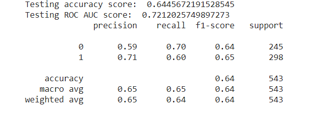
We ran a Logistic Regression model (courtesy of the sklearn library) with a maximum of 10,000 iterations until convergence. The accuracy score on the test data was around 64.46%, and the ROC-AUC (Area Under the Receiver Operating Characteristics) score was 72.12%. To be more specific, the classification report is as follows. For “not hit”, we achieved a precision score of 59% and a recall score of 70%, while for “hit”, we achieved a precision score of 71% and a recall score of 60%.

Naive Bayes

We also tried using naive Bayes to classify songs as either a hit or not a hit (using the same rule as for logistic regression). First, to reduce the number of features being used, we used k-best feature selection, with the scoring metric being an analysis of variance. (We also tried using χ^2, but this was not suitable as loudness values are stored in decibels (dB), which can be negative.) Using these features, we used sklearn’s GaussianNB class to test the model, with 80% of the data being used for training and 20% for testing. Before adding in the artist familiarity and hotness values to the dataset, using 4-best feature selection led to us using the key, mode, tempo, and time signature to predict whether or not a song was a hit with ~55.5% accuracy.

Once we added in artist hotness and familiarity, using 4-best feature selection led to us using the mode, tempo, artist’s hotness, and artist’s familiarity to predict whether or not a song was a hit with 72.45% accuracy. Tweaking the number of features selected does not substantially affect the accuracy of the model:

k	feature added to the model	accuracy
1	artist hotness	69.71%
2	artist familiarity	72.72%
3	mode	71.56%
4	tempo	72.45%
5	time signature	71.92%
6	key	72.01%
7	loudness	72.63%
8	duration	72.80%

(Note that since we are selecting the k best features at each stage, the “feature added” column in the table above is cumulative. So, for example, for k = 3, the model included artist hotness, artist familiarity, and mode.)

We can see that while naive Bayes technically does best when given all eight of these features, the difference is almost imperceptible when compared to naive Bayes based simply on artist hotness and artist familiarity.

Neural Networks:

Unfortunately, no matter how we tweaked the number of layers, input features, and activation functions, we were not able to achieve an accuracy higher than 69.5%, which was worse than naive Bayes.

Unsupervised Learning

K-Means:

Below we have the graphs for the elbow method and the silhouette value from 2 clusters up to 14 clusters when using K-Means on the dataset including timbre data

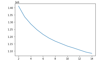
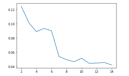
As we can see, the silhouette coefficient continually decreases as the number of clusters increases, and the elbow graph is not entirely clear on where the optimal point should be, leading us to conclude that the optimal value for k is just 2 clusters. This doesn’t really fit our data because we have 13 genre labels, so theoretically if the model were to classify genres well, it should have 13 clusters.

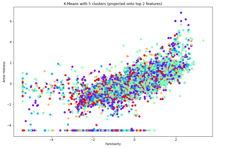
To illustrate the model, we generated a scatter plot of the points and their 13 clusters projected onto the top 2 features, which were familiarity and artist hotness.

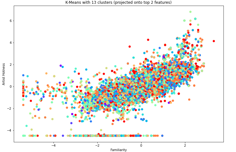
Visually we can see that 13 clusters doesn’t seem to work very well. From the silhouette graph, the next best k value seems to be 5 since we don’t really want to use 2, so we investigate using 5 clusters to see if the model groups genres together within the clusters.

Not too much better, but at least consistent with the silhouette values.

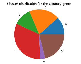
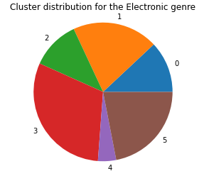
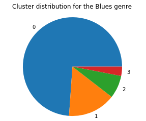
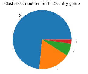
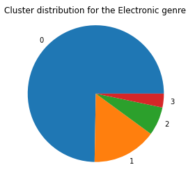
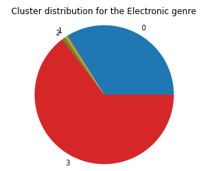
We graphed the genre distribution across the 5 clusters and the graphs for the Blues, Country, and Electronic Genre are below:

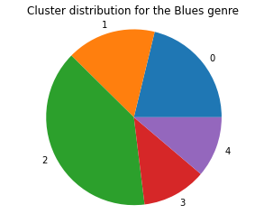
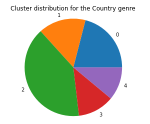
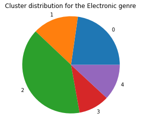
The pie charts for all the other genre distributions are all very similar, telling us that the k-means model doesn’t do a very good job of clustering based on genre. We then run the k-means model on the control dataset without the timbre data

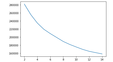
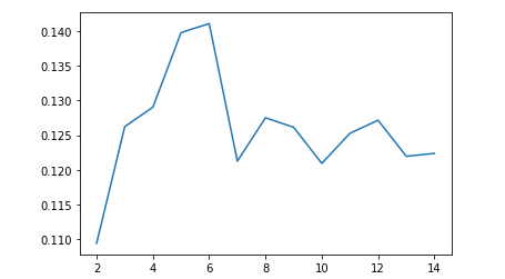
As we can see, the elbow method is once again a little unclear. When we visualize the silhouette values, we see that 6 clusters seems to be the optimal number of clusters for this k-means model. Next we visualize the clusters over the top 2 features, still familiarity and artist hotness.

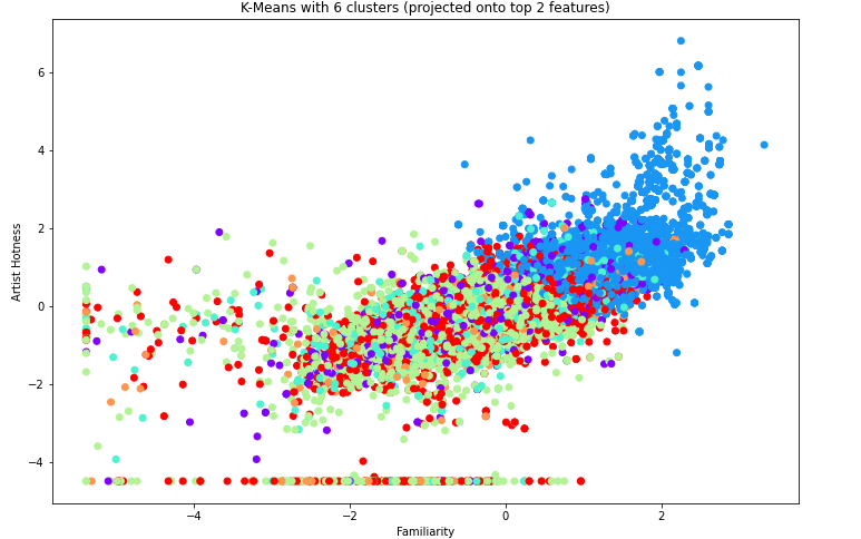
We can see that when using the dataset without the timbre, we begin to see visual representation of clusters, such as the blue points on the above graph.

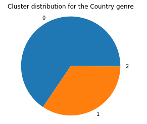
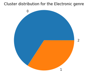
Next, we graphed the genre distribution across the 6 clusters, and the graphs for the Blues, Country, and Electronic Genre are below:

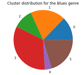
As we can see, it doesn’t seem that the k-means model clusters based on genre, but from the 2D approximation of the clusters, it is clear that it is clustering on some other underlying criteria. This leads us to believe that the data in the MSD, when ignoring the genre tags, doesn’t tell us much about the genre of the song, or that there is some other underlying criteria that separates groups of songs from one another that is stronger than genre classifications.

GMM:

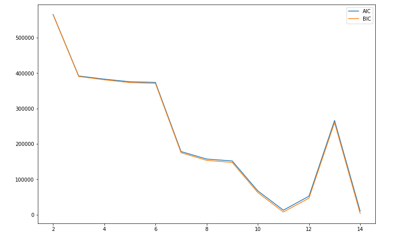
Below we have the graphs for the elbow method from 2 components up to 14 components when using GMM on the dataset including timbre data. For the error, we graphed Akaike’s Information Criteria (AIC) and Bayesian Information Criteria (BIC) so that we could see both and use them to determine the optimal number of components. We anticipate that this model will work better than k-means because in GMM, the components need not be spherical:

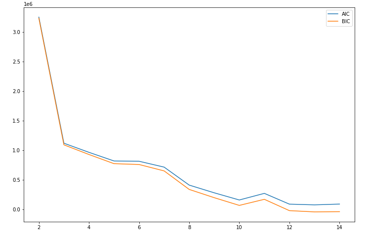
From this graph, we took the optimal number of components to be 4, and we then visualized the clusters from GMM by projecting onto the top 2 features, once again familiarity and artist hotness.

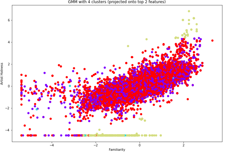
We can kind of see the clusters forming, which is promising. To see if these clusters mean anything in terms of genre classification, we graph the cluster distributions for each genre, and the graphs for Blues, Country, and Electronic are as follows:

As we can see, once again, the data doesn’t seem to be clustering based on genre since the cluster distributions are roughly equivalent across all genres.

Next we ran the GMM model on the dataset excluding the timbre features. The elbow graph is as follows:

This graph was a little hard to interpret, so we also calculated the silhouette values for these numbers of components. The silhouette values are as follows:

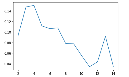
From these silhouette values, we see that the optimal number of clusters seems to be 4. We visualized the 4 clusters below.

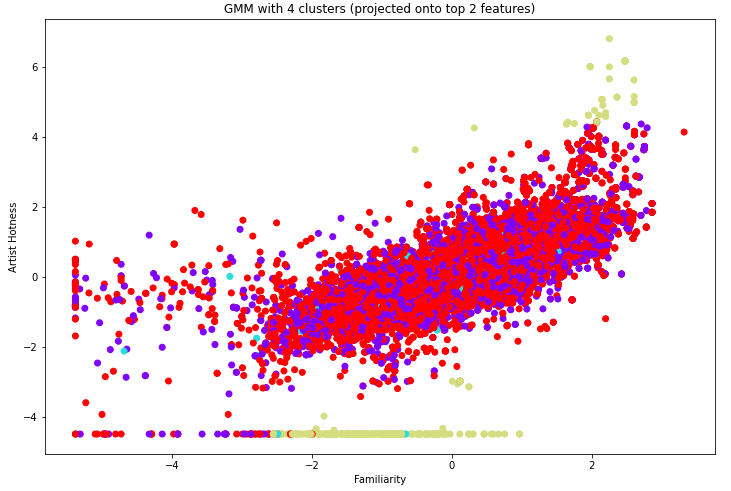
We can kind of see clusters forming here. It seems like the red and purple clusters are intermingled here, but remember that this is only a 2D approximation over the top 2 features; the red and purple clusters could be completely separate if we could visualize more dimensions. To see if these clusters mean anything in terms of genre classification, we visualized the cluster distributions for each genre. The pie charts for Blues, Country, and Electronic are shown below.

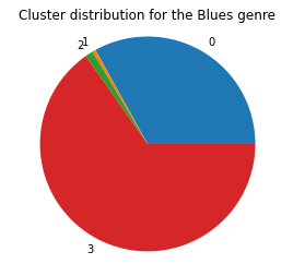
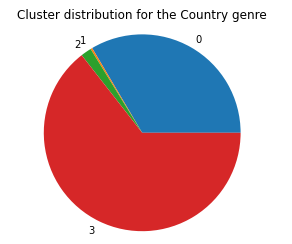
As before with k-means, it seems that the GMM model is also unable to cluster based on genre, further suggesting that there is some underlying criteria among the data features that delineates group of songs more than genre does. With GMM, the clusters do not have to be spherical and can therefore de-emphasize features that do not contribute much to the classification, but even with this improvement over k-means, the data does not inherently cluster based on genre.

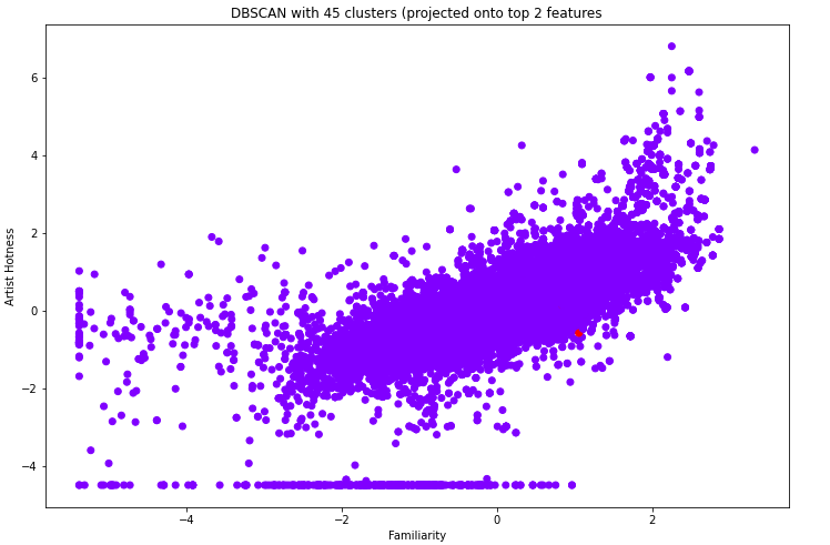
DBScan:

For the dataset with timbre, running DBScan resulted in either one large cluster encompassing the entire dataset or many, many small clusters that were pretty much each core sample and its immediate neighbors. This is within expectation because there were much more timbre features than metadata features (36 vs 9), leading to the timbre features dominating. Since DBScan clusters are distance based, this leads to the timbre features dominating the distance calculation, making all of the songs seem to belong to one cluster since the remaining 9 features cannot do much to impact the distance calculations. An example of DBScan resulting in 1 giant cluster and some outliers is shown below.

We then ran DBScan on the dataset without any timbre features. With `eps=2` and `min_samples=10`, we were able to get a model with 3 clusters as follows.

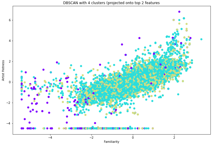
To see if these clusters mean anything in the context of genre classification, we again visualize the cluster distributions per genre, with Blues, Country, and Electronic being shown below.

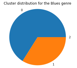
As we can see, the cluster distributions are rather uniform across all genres once again, meaning that DBScan is clustering on some other underlying criteria within the data features that delineates groups of songs better than the genre does. Using the song metadata as a dataset to cluster songs does not lead to genre classification.

Discussion on unsupervised learning portion:

It seems that the clustering models do not work well for genre classification. Clustering on the song metadata provided in the Million Song Dataset does not seem to reveal anything about the genres of the songs themselves, and even when using the timbre features that were selected as detailed above, there was no meaningful improvement in the performances of the models that we tried (K-Means, GMM, and DBScan). Perhaps this problem would be better suited on a dataset that contains the song audio data or some sample of the audio data. However, clusters did appear when clustering on the features we had; they just didn’t cluster with respect to genre. This implies that we could possibly figure out the unknown criteria that the data is actually being clustered on, which may give insights what makes songs different from one another.

Conclusions

Supervised Learning:

Our results for hit prediction did fare better than random chance (at 72.8% accuracy), but the results depend heavily on whether the song’s artist is well-known. Without the artist data, the accuracy drops to 55.9%, which is barely better than flipping a coin. As such, they make this model essentially useless for predicting whether an up-and-coming artist’s song will become a hit. Nonetheless, these results may actually be reassuring for the general public, as they seem to refute the widely-held notion that pop music is increasingly bland or formulaic. A more thorough analysis of the features we ignored in our supervised learning models (such as timbre data) may be needed to solidify that conclusion, but the features we analyzed cover many of the important features of a song (like its tempo, time signature, key signature, and mode) that define its character.

Unsupervised Learning:

It seems that the clustering models do not work well for genre classification. Clustering on the song metadata provided in the Million Song Dataset does not seem to reveal anything about the genres of the songs themselves, and even when using the timbre features that were selected as detailed above, there was no meaningful improvement in the performances of the models that we tried (K-Means, GMM, and DBScan). Perhaps this problem would be better suited on a dataset that contains the song audio data or some sample of the audio data. However, clusters did appear when clustering on the features we had; they just didn’t cluster with respect to genre. This implies that we could possibly figure out the unknown criteria that the data is actually being clustered on, which may give insights what makes songs different from one another. The next steps would have been to explore if the clustering model worked for song recommendations; unfortunately, the website containing the documentation on how to use the API for user data returns a 404 error, as well as the website that would generate a token to give us permissions to use the data, so even if we could reason the API functions from the source code, we were unable to access the EchoNest user playlist data that accompanies the Million Song Dataset. Maybe if we have a way to generate a token later on, or have the resources to create our own dataset of user playlists, we could continue investigating if the clustering models are still useful for song recommendations even if they do not cluster based on genre.

Group Members

Sahir Shahryar: Data Collection, Supervised Learning, Final Video

Leonardo Tang: Unsupervised Learning, Supervised Learning, Website

Our group quickly went down to 2 people after initially having 4 after the project group formation, so this has been a 2 person final project for effectively the entire lifetime of the project

References

[1] He, Hui, Jianming Jin, Yuhong Xiong, Bo Chen, Wu Sun, and Ling Zhao. Feature Mining for Music Emotion Classification via Supervised Learning from Lyrics. International Symposium on Intelligence Computation and Applications, 2008.

[2] Li, Tao, and Mitsunori Ohigara. Music artist style identification by semi-supervised learning from both lyrics and content. Proceedings of the 12th annual ACM international conference on Multimedia, October 2004.

[3] Million Song Dataset. An example track description.

[4] Lamere, Paul. Artist similarity, familiarity, and hotness. May 25, 2009.

[5] Dhillon, Guan, and Kulus. Kernel k-means, Spectral Clustering and Normalized Cuts.

[6] Jie and Han. A music recommendation algorithm based on clustering and latent factor model.

[7] Tyagi and Wellekens. On desensitizing the Mel-cepstrum to spurious spectral components for robust speech recognition.